Remove Duplicate Rows
Using this tool, you can remove duplicate rows from your data.
To use this tool, click on the “Remove Duplicate Rows” option under the “Dedupe & Compare” section. Once you have the “Remove Duplicate Rows” page open, you can follow the steps below:
Step-1:
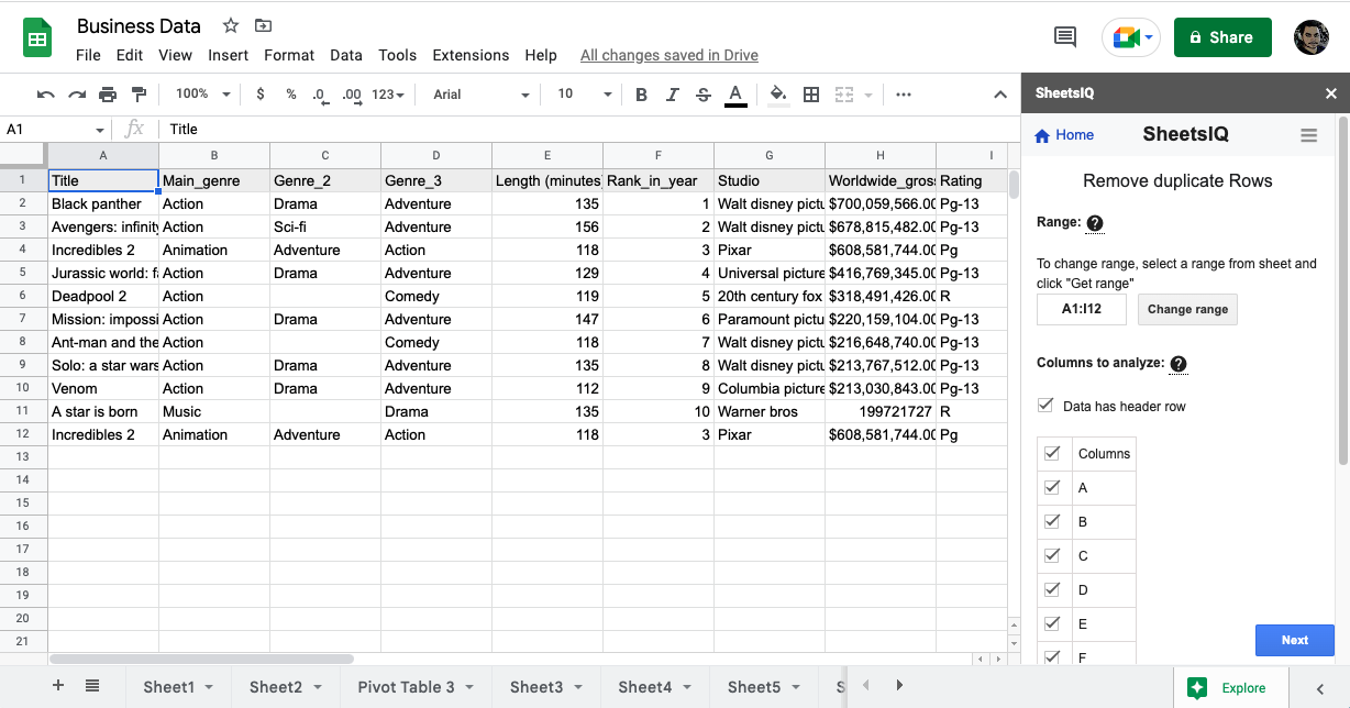
Select Range: By default the current data range of the sheet will be selected and will show up under the range.
You can change this by either selecting a range from the sheet and clicking on the “Change range” button or manually typing the range. Preferred way is the first one.
Columns to analyze:
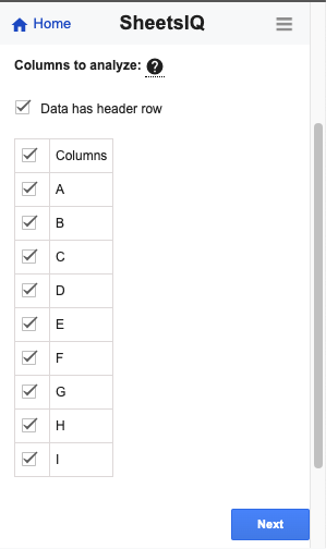
Here you will select the columns which will be included while checking for duplicates.
By default the entire data range is selected and you will see all the columns in the data range listed and check marked. You can choose to uncheck the ones that are not required.
Click on the “Next” button to go to step-2.
Step-2:
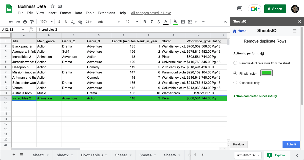
In this step, you need to choose the action you want the tool to perform when duplicate rows are found.
You can either
- Remove the duplicate rows from the sheet
- Highlight the duplicate rows with color
- Clear cells in the duplicate rows
In this example, I want to highlight the duplicate cells with green color.
So first I will choose the option “Fill with color” and then select the green color by clicking on the color picker.
Finally, click on the “Apply” button to see the result.
Remove duplicate cells
Using this tool, you can remove or highlight duplicate cells in your data.
To use this tool, click on the “Remove Duplicate Cells” option under the “Dedupe & Compare” section. Once you have the “Remove Duplicate Cells” page open, you can follow the steps below:
Step-1:
Select Range: By default the current data range of the sheet will be selected and will show up under the range.
You can change this by either selecting a range from the sheet and clicking on the “Change range” button or manually typing the range. Preferred way is the first one.
In this example, my data is in the range of A17 to B24, so I will select the range and click on “Get Range” button to select the range.
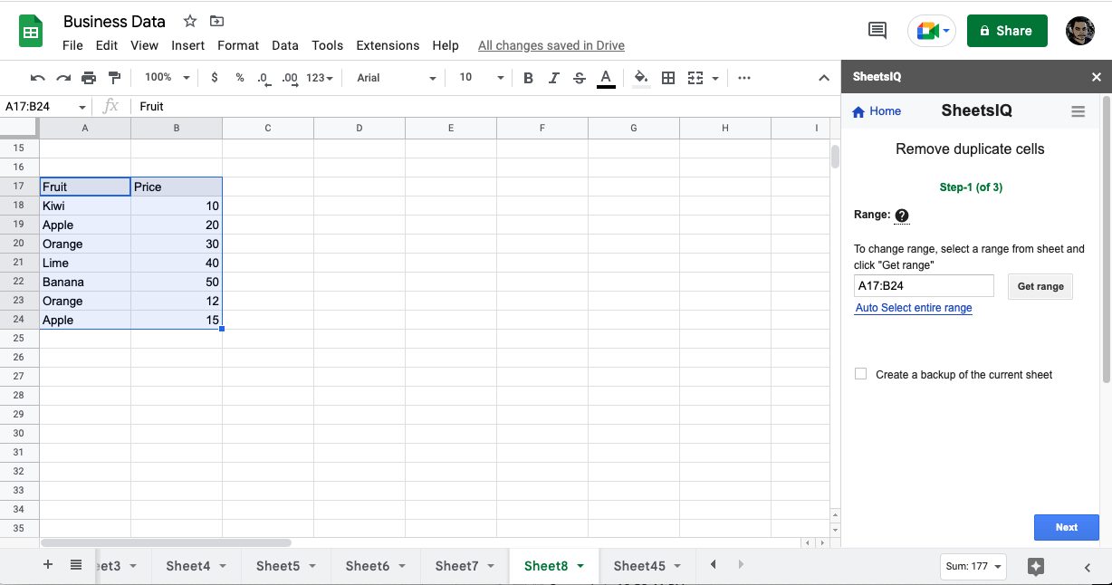
Click on the “Next” button to go to the next step.
Step-2:
In this step, you need to tell the tool if you want to find “Duplicates” or “Uniques”. By default “Duplicated” is selected.
Duplicates refer to any duplicate cell in the range. The tool will start looking at all cells one by one starting from the top left cell till the bottom right cell. While going through from top to bottom, if a cell value is repeated anywhere then the tool will mark it as duplicate.
Uniques refer to all unique cell values in the range.
You can choose additional options like whether or not to skip empty cells and match cases while the tool searches for duplicates or uniques.
For this example, I will leave the default selections and click on the “Next” button.
Step-3:
Here you can choose the action to perform when the tool finds duplicate or unique cells.
Fill with color - This will fill the duplicate or unique cells with the selected color from the color picker.
Clear values - This will clear the values of the duplicate or unique cells.
Copy to another location - This will copy the result to a desired location as per the options you choose.
Move to another location - This will move the duplicate or unique cells to a desired location as per the options you choose.
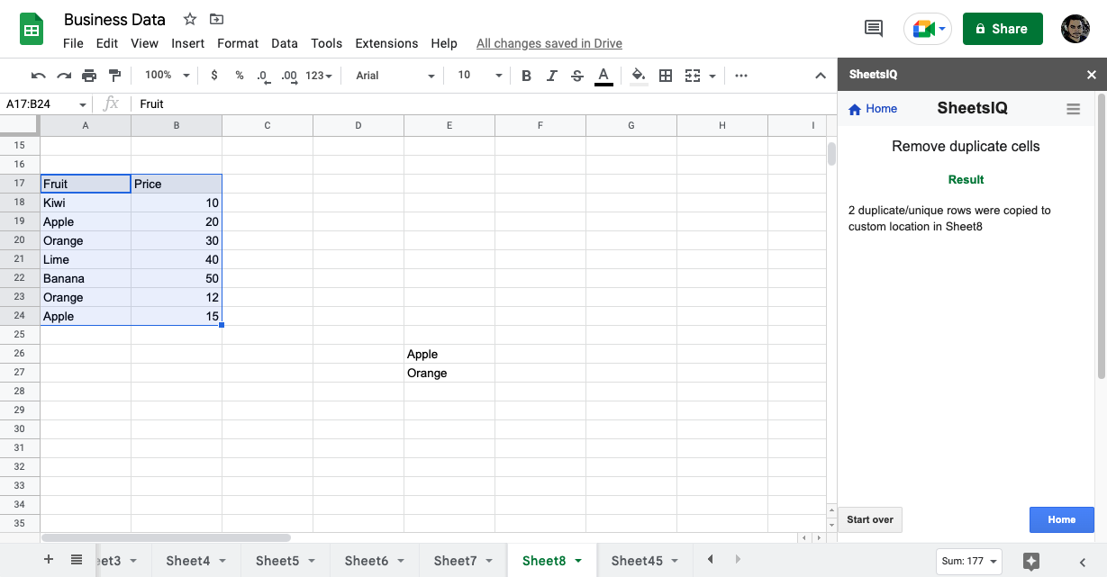
In this example, I want to copy the duplicate cells to the bottom of the current sheet.
So I will select the “Copy to another location” option. Then under the sub-section, I will choose “Custom location”. In the range field, I will type E26.
(You need to type or select the first cell for the custom location and the tool will automatically fill the result from that cell onwards)
Now click on the “Apply” button and check the result.
Compare Columns and Sheets
Using this tool, you can compare data between two columns or sheets and find duplicates or unique values in the first sheet.
To use this tool, click on the “Compare Columns & Sheets” option under the “Dedupe & Compare” section. Once you have the “Compare Columns & Sheets” page open, you can follow the steps below:
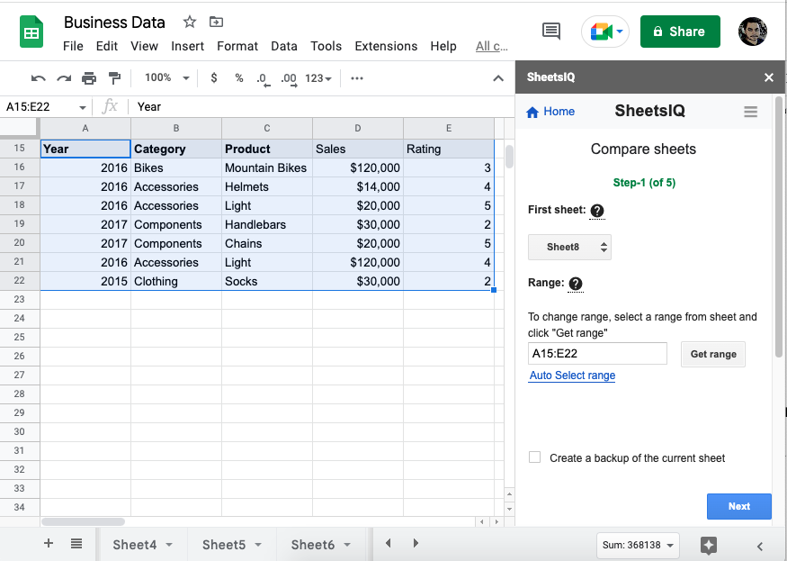
Step-1:
Select first sheet:
By default when the “Compare Columns & Sheets” page loads, it will select the current sheet. You can choose to select a different sheet from the current spreadsheet from the drop-down option.
Select Range: By default the data range of the selected sheet will show up under the range.
You can change this by either selecting a range from the sheet and clicking on the “Change range” button or manually typing the range. Preferred way is the first one.
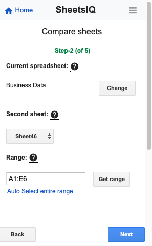
Step-2:
Select second sheet:
In this step, you need to provide the second sheet details.
Note:- By default the tool will select the next sheet of the same spreadsheet.
Current spreadsheet -
By default the current spreadsheet is selected. The name of the current spreadsheet will show. You can change this to a desired spreadsheet from the google drive.
To change, click on the “Change” button. This will bring a popup on the screen where you can enter the url of the second spreadsheet from your drive.
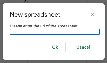
(Make sure you are providing the spreadsheet from your own google drive that is associated with the same email account that you have used to access this add-on in the current spreadsheet)
The URL of a google sheets looks like this:
Note the highlighted part. This you need to paste in the popup.
Once you do, click Ok and the spreadsheet name will change to the newly added spreadsheet.
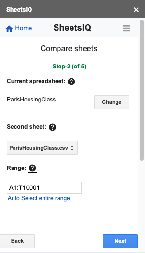
For this example I am using the same spreadsheet as step-1.
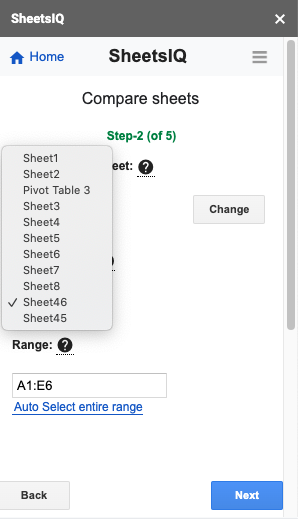
Second sheet -
All the sheets from the spreadsheet will appear here. You can choose to select any sheet from the drop down.
Range -
The range will be auto selected based on the sheet you select. You can change the range.
You can change this by either selecting a range from the sheet and clicking on the “Change range” button or manually typing the range. Preferred way is the first one.
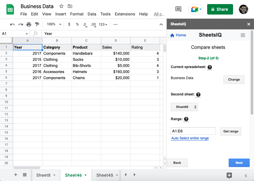
Here is step-2 of this example.
Step-3:
In this step, you need to tell the tool if you want to find “Duplicates” or “Uniques”. By default “Duplicated” is selected.
Duplicates refer to any duplicate cell in the range. The tool will start looking at all cells one by one starting from the top left cell till the bottom right cell. While going through from top to bottom, if a cell value is repeated anywhere then the tool will mark it as duplicate.
Uniques refer to all unique cell values in the range.
For this example, I am finding duplicate values.
Step-4:
In this step, you will select the columns of both sheets that will be compared by the tool to find duplicates or uniques.
Select columns to compare -
If the data in the first sheet has a header, then tick the checkbox for “Table 1 has header”.
If the data in the second sheet has a header, then tick the checkbox for “Table 2 has header”.
Skip empty cells : By default the tool will skip empty cells. If you want to count the empty cells as duplicates or uniques, then you can turn this off.
Match case: If you enable this, then the tool will match the case of cell value while comparing cell values for finding duplicates or uniques.
For this example, since I have headers in both the sheets, I will check to mark both “Table 1 has header” and “Table 2 has header”.
I will leave the other 2 options to default values.
Map Table 1 columns with Table 2:
Choose columns to compare:
First thing is to decide what we are comparing between the two tables. We will only check these columns to proceed.
Case-1: If you want to compare the complete row of Table1 with Table2, then you will check mark all the columns.

In this case, the tool will check if any of the rows in Table1 exist in Table2.
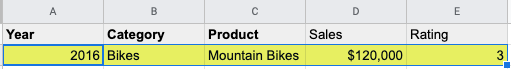
(Yellow highlight is for example only. This shows that entire row will be considered when finding duplicates)
Case-2: You may need only certain column combinations to compare. For example, you may want to see if there is a duplicate product in Table2. So you will only check mark the C column.

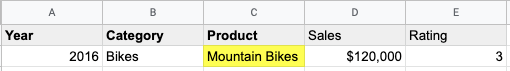
(Yellow highlight is for example only. This shows that only column C values will be considered when finding duplicates)
If you need to see category and product combination to be checked, then choose column B and C. Now the tool will compare if Category and Product both exists in second sheet.
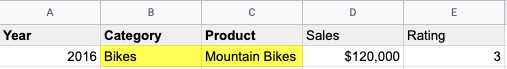
(Yellow highlight is for example only. This shows that only the combination of Column B and column C will be considered when finding duplicates)
Map the columns
Once you decide which columns to check, next you will select the mapping between Table 1 and Table 2.
Let’s understand this by an example.
Table 1 has below columns,

Table 2 has below columns,

If this is the case, then the mapping will be:
Table1 Column A = Table2 Column A
Table1 Column B = Table2 Column B
Table1 Column C = Table2 Column D
Table1 Column D = Table2 Column C
Table1 Column E = Table2 Column E
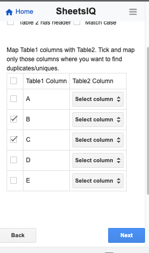
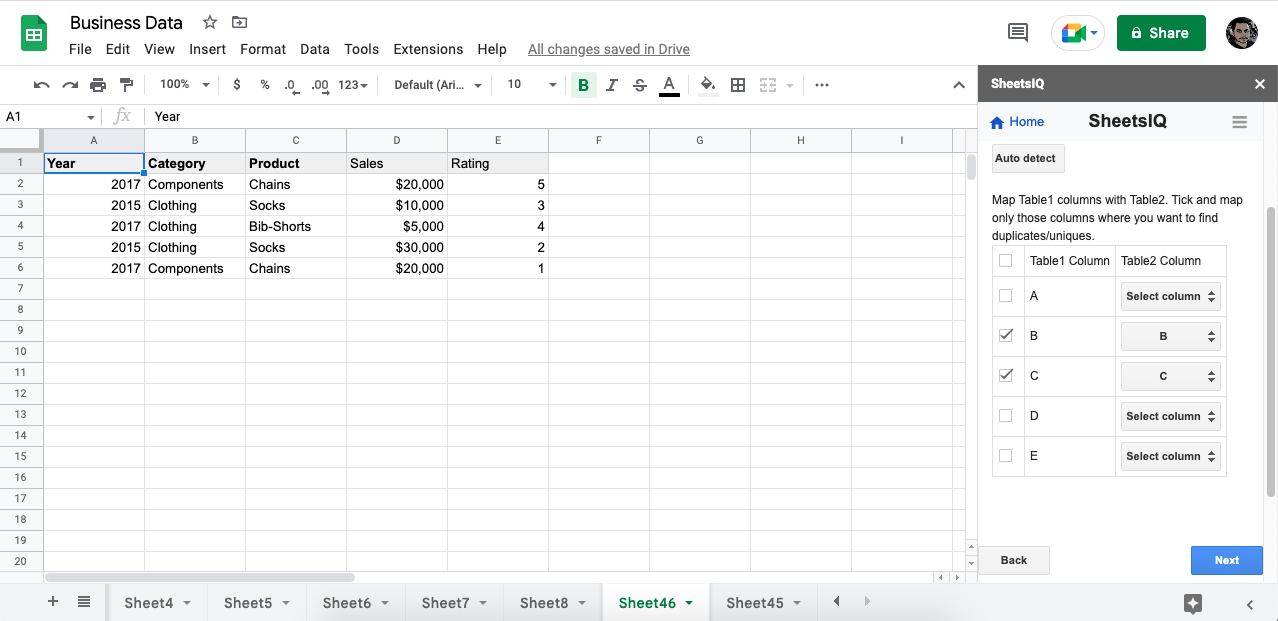
In the current example that we are working on, I want to compare category and product combinations.
So I will check the box for column B and column C. Then I will map them with column B and column C of the second sheet respectively.
This is how the step-4 looks like:
Step-5:
In this step, you will select the action to perform after finding duplicates or uniques.
Fill with color - This will fill the duplicate or unique cells with the selected color from the color picker.
Add status column - This will add a status column next to the last column of Sheet1. The status column will mention “Duplicate” for duplicates and “Unique” for uniques.
Clear values - This will clear the values of the duplicate or unique cells.
Delete entire row from the sheet - This will delete the duplicate/unique row from Sheet1.
Copy to another location - This will copy the result to a desired location as per the options you choose.
Move to another location - This will move the duplicate or unique cells to a desired location as per the options you choose.
In this example that you are following, I just want to highlight the duplicates. So I will choose the first option which is by default selected.
Next, click on the “Apply” button.

As you can see, the rows having the duplicates have been highlighted.
Combine Duplicate Rows
Using this tool, you can combine duplicate rows in your data.
To use this tool, click on the “Combine Duplicate Rows” option under the “Dedupe & Compare” section. Once you have the “Combine Duplicate Rows” page open, you can follow the steps below:
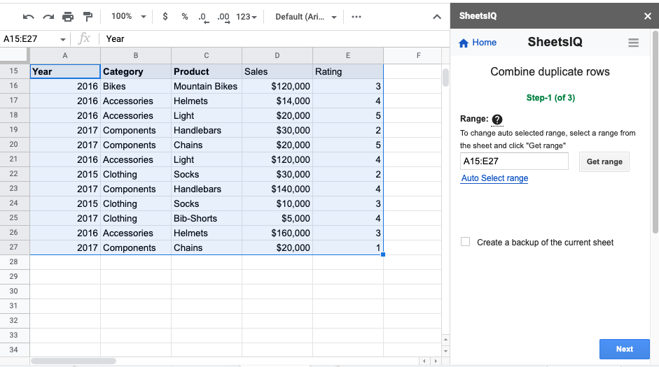
Step-1:
First you need to select the range of data to work on.
By default when the “Combine Duplicate Rows” page loads, the data range of the current sheet will show up under the range.
You can change this by either selecting a range from the sheet and clicking on the “Change range” button or manually typing the range. Preferred way is the first one.
Step-2:
In this step, you need to choose the columns which will be considered while checking for duplicates.
Data has header row - Tick this if you have a header row in your data and that will not be considered while searching for duplicates.
Skip empty cells - This will ensure that empty cells are not considered while finding duplicates.
Match case - If you tick this box, then the tool will consider the case of cell value while finding duplicates.
Select columns where you want to find duplicates:
Select only those columns which need to be considered for checking duplicates.
In this example, I am checking duplicates for Category and Product combinations. I.e if Accessories + Helmet will have duplicate entries, I want to know that.
So I will select column B and column C.
Also I will tick the box for “Data has header”, as I have a header row.

Click on the “Next” button.
Step-3:
In step-2 we selected the columns where we want to find duplicates. In this step, we will decide how to combine the remaining columns while merging the duplicate rows.
I had selected column B and column C in step-2. So in this step, I have the option available for column a, column D and column E for combining.
I want to add the sales values while combining the duplicates.
So I will first tick mark the box column D. Under Action, I will select “Calculate” and under Function I will select “SUM”.

Now I will click on the “Submit” button.
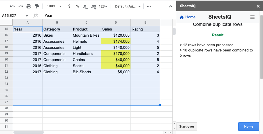
You can see that the duplicate rows were deleted. Sales values were combined.
Quick Dedupe
Using this tool, you can perform advance dedupe in one step.
To use this tool, click on the “Quick Dedupe” option under the “Dedupe & Compare” section. Once you have the “Quick Dedupe” page open, you can follow the steps below:
Range -
First you need to select the range of data to work on.
By default when the “Quick Dedupe” page loads, the data range of the current sheet will show up under the range.
You can change this by either selecting a range from the sheet and clicking on the “Change range” button or manually typing the range. Preferred way is the first one.
Data has header - Check this box if you have a header row in your range.
Skip empty cells - By default it is checked, i.e the tool will not consider empty cells while checking duplicates.
Match case - Check this box if you want to consider the case of the cell text while checking for duplicates.
Tick columns where you want to find duplicates -
By default all columns are checked. This means that the tool will check if the entire row has duplicate entries.
If you uncheck some of the columns, then the tool will check if the combination of checked columns in a row has duplicate entries.
Choose the action -
Here you can choose the action that will be performed once duplicates are found.
You can:
- Fill the duplicate row with color
- Delete the duplicate row
- Add a status column marking it as “Duplicate”
- Clear values of duplicate row
- Copy to new sheet will copy the duplicate rows to a new sheet (Link of new sheet will be provided at the result page)
- Move to new sheet will move the duplicate rows to a new sheet (Link of new sheet will be provided at the result page)
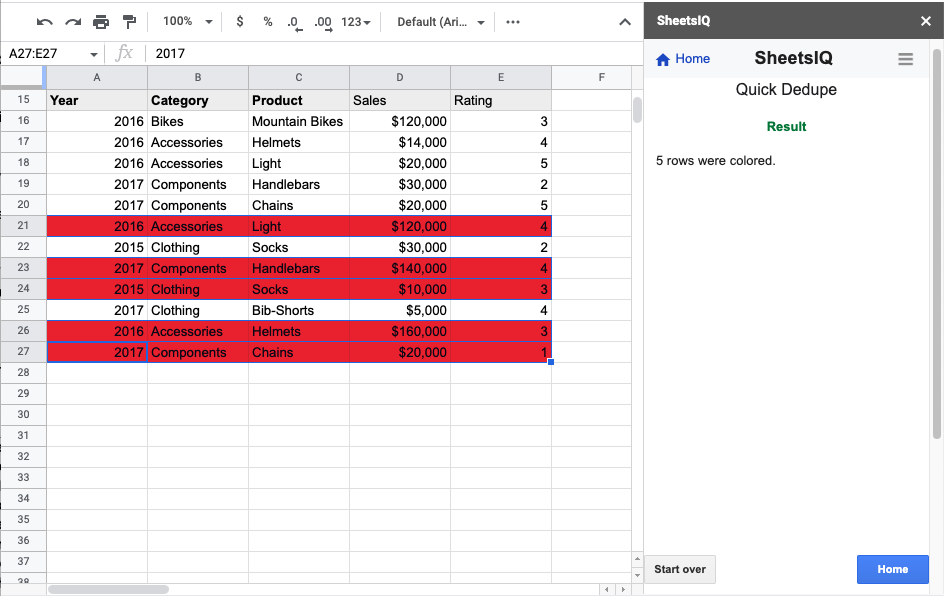
In this example, I want to consider column B and column C as a combination to find duplicates. Basically, I want to highlight Category+Accessories duplicates.
Here is my setting.
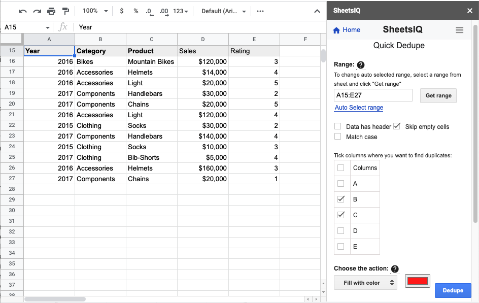
After I click on the “Apply” button, you can see the duplicates getting highlighted.