Merge values
Using this tool, you can merge values in a range with advanced options and customization.
To use this tool, click on the “Merge Values” option under the “Merge & Combine” section. Once you have the “Merge Values” page open, you can follow the steps below:
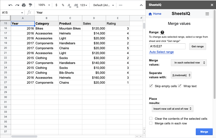
Range -
First you need to select the range of data to work on.
By default when the “Merge Values” page loads, the data range of the current sheet will show up under the range.
You can change this by either selecting a range from the sheet and clicking on the “Change range” button or manually typing the range. Preferred way is the first one.
Merge values -
Choose how you want to merge values. You can:
- into one cell - All values of the range will be merged as one cell
- In each selected rows - All values in each row will be merged
- In each selected columns - All values in each column will be merged
Separate values with -
You can choose to add a delimiter while merging multiple cell values.
You can have semicolon, comma, space or line break added while merging cell values.
Skip empty cells - This will skip empty cells while merging
Wrap text - This will wrap the text in the merged cell
Place results - You can choose where to put the result.
Clear content of the selected cells - If you check this then after merging all cells of the range will be cleared
Merge all selected cells into one - If you check this then all cells in the range will be merged into one cell. If this is unchecked, then after merging all cells in the range and placing them at say “top left corner”, remaining cells of the range will remain as is. Default value is unchecked.
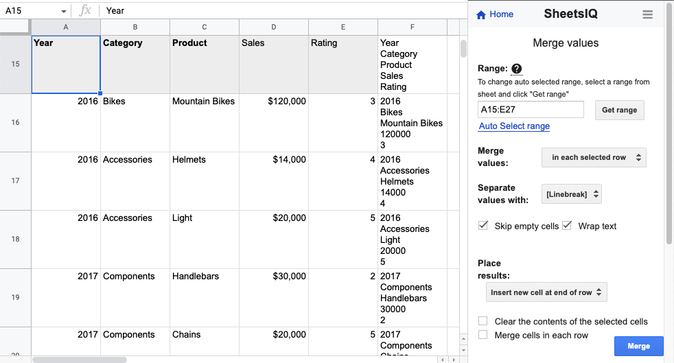
In this example, I want to merge all values in each row, separate them by line break and put the result in a new cell at the end of each row. Here is my setup:
Now once I click on the “Apply” button, you can see the result:
Merge sheets
Using this tool, you can merge sheets into one using advanced options.
To use this tool, click on the “Merge Sheets” option under the “Merge & Combine” section. Once you have the “Merge Sheets” page open, you can follow the steps below:
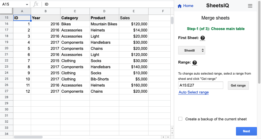
Step-1:
First Sheet -
Here you need to provide the first sheet name to the tool. By default the current sheet is selected. You can choose to change this to any sheet in the current spreadsheet.
Range -
By default when the “Merge Sheets” page loads, the data range of the current sheet will show up under the range.
You can change this by either selecting a range from the sheet and clicking on the “Change range” button or manually typing the range. Preferred way is the first one.
Here is my step-1 for this example.
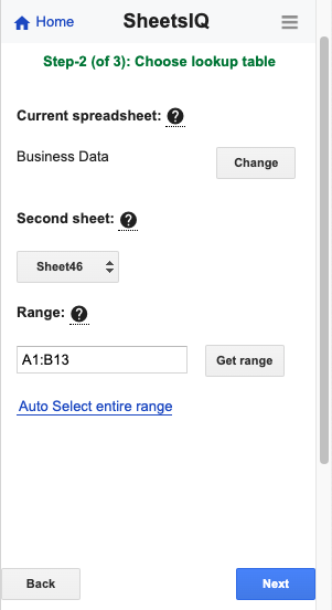
Step-2:
Select second sheet:
In this step, you need to provide the second sheet details.
Note:- By default the tool will select the next sheet of the same spreadsheet.
Current spreadsheet -
By default the current spreadsheet is selected. The name of the current spreadsheet will show. You can change this to a desired spreadsheet from the google drive.
To change, click on the “Change” button. This will bring a popup on the screen where you can enter the url of the second spreadsheet from your drive.
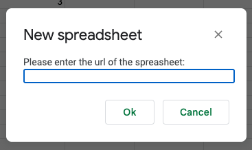
(Make sure you are providing the spreadsheet from your own google drive that is associated with the same email account that you have used to access this add-on in the current spreadsheet)
The URL of a google sheets looks like this:
Note the highlighted part. This you need to paste in the popup.
Once you do, click Ok and the spreadsheet name will change to the newly added spreadsheet.
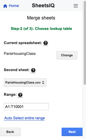
For this example I am using the same spreadsheet (Business Data) as step-1.
Second sheet -
All the sheets from the spreadsheet will appear here. You can choose to select any sheet from the drop down.
Range -
The range will be auto selected based on the sheet you select. You can change the range.
You can change this by either selecting a range from the sheet and clicking on the “Change range” button or manually typing the range. Preferred way is the first one.
Here is the step-2 of this example.
Step-3:
In this step, you will choose how to merge data.
Merge action -
Option-1: Just move the data
If you choose this option, then the data from sheet2 will be copied to sheet1 and the data will be either placed to the right or at the bottom of the current sheet range.
Option-2: Move & Update data
If you choose this option, then the data will be moved from sheet2 to sheet1 and sheet1 data will be updated.
Map unique column - While moving data from sheet2 to sheet1, to update sheet1 data, the tool needs an unique column. Unique column is a column that is unique in both sheets. Example, if you have data about transactions of an online store, then the transaction ID will be unique.
How this works : Tool will take the unique column value from sheet1, search for same in sheet2 and based on the result found, the tool will move data and update from sheet2 to sheet1.
Place result - Here you can define whether you want to update sheet1 or create a new sheet with the merged data.
For this example we are following, I want to move and update the data. My unique data is the ID column which is in column A in both sheets.
So here is the step-3 example:
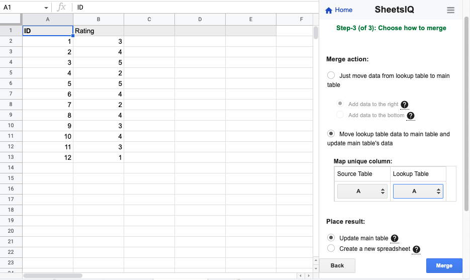
Now if I click on the “Merge” button, the tool will merge the sheets and bring data to sheet1.

Combine sheets
Using this tool, you can combine sheets into one using advanced options. You can combine more than two sheets using this tool.
To use this tool, click on the “Combine Sheets” option under the “Merge & Combine” section. Once you have the “Combine Sheets” page open, you can follow the steps below:
Problem:-
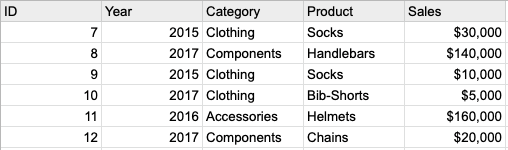
I have three sheets with the below data.
Sheet1:-

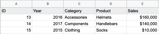
Sheet2:-
Sheet3:-
I want to combine these to get this:-
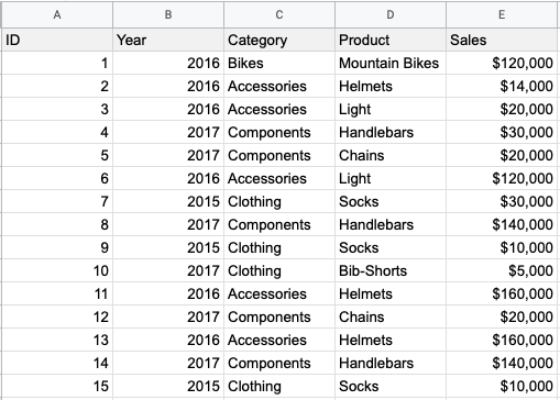
Let’s see how to achieve this.
Step-1:
In this step, you will select the sheets to combine.
You can combine sheets from the same spreadsheet or different spreadsheets of your google drive.
By default the current spreadsheet is listed. You can add a new one by clicking “Add from drive”.
This will bring a popup on the screen where you can enter the url of the second spreadsheet from your drive.
(Make sure you are providing the spreadsheet from your own google drive that is associated with the same email account that you have used to access this add-on in the current spreadsheet)
The URL of a google sheets looks like this:
Note the highlighted part. This you need to paste in the popup.
Once you do, click Ok and the new spreadsheet name will appear on the screen with its list of sheets.
For this example, my sheets are in the same spreadsheet. So I will click on the expand arrow to view all sheets and select the sheets that contain my data.
Here is my step-1:

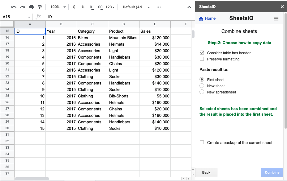
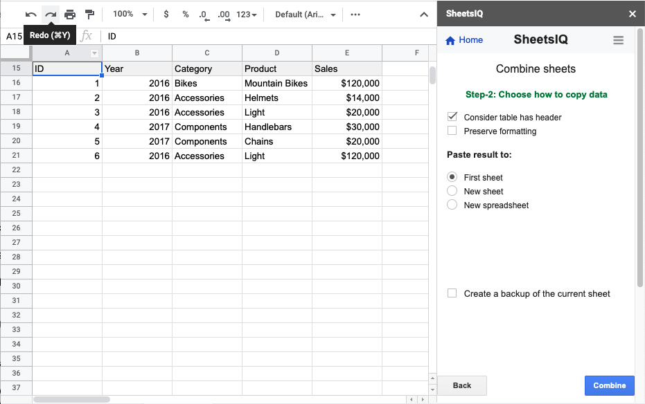
Step-2:
In this step, you will choose how to copy data.
We strongly suggest having headers in all sheets. This will make the move uniform.
Consider table has header - Check this to let the tool know that you have header rows in your sheets.
Preserve formatting - Check this if you want to preserve the formatting while moving the data.
Paste result to -
Choose where to paste the result. You can:
- Paste it in the first sheet
- Paste in a new sheet
- Paste in a new spreadsheet (Link will be shared at the result page)
Here is my step-2:
Now click on the “Combine” button.
Here is the result: