Do you want to evaluate multiple conditions using nested if statements in google sheets?
Here I will show you all information about how to write nested if statements in google sheets. Also I will show you how you can simplify it using the IFS formula.
Nested IF statements in google sheets
Here is how to write nested if statements in google sheets:
=IF(logical_expression, value_if_true, IF(logical_expression2, value_if_true2, IF(logical_expression3, value_if_true3, value_if_false)))
As you can see, there are multiple IF statements that are nested together.
First IF statement evaluates if the “logical_expression” is TRUE. If it is TRUE then it outputs “value_if_true“.
Else, it will look for the second IF statement and evaluate the “logical_expression2“. If the evaluation results TRUE then it will output “value_if_true2” else it will move to the next IF statement and so on.
Example – Nested IF statements in google sheets
Let’s say you have a data set from an e-commerce website. You have traffic, orders and conversion rates of different product pages listed in a table.
Here is the data:-
| Landing Page | Traffic | Orders | Conversion Rate |
| Lead page | 5000 | 180 | 3.60% |
| Product page | 5000 | 140 | 2.80% |
| Blog page | 4000 | 250 | 6.25% |
| Home Page | 2000 | 10 | 0.50% |
Here is what you want:-
If the conversion rate is below 1% then analyse that web page Today.
If the conversion rate is between 1 to 2% then do it tomorrow.
For 2-4% do it on Thursday and for <10% do it on Friday.
Using nested if statements in google sheets, you can solve this. Here is the formula:
=IF(D2<1%,"Today",IF(D2<2%,"Tomorrow", IF(D2<4%,"Thursday",IF(D2<10%,"Friday","Error"))))And here is the final result:
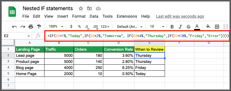
So this is how you use nested if statements in google sheets.
But there is a better way to write this using the newly introduced IFS formula.
Here is how:
IFS Formula – Alternative to nested if statements in google sheets
Syntax
Here is the syntax for the IFS function that helps to nest multiple IF statements.
= IFS(condition1, value1, [condition2, value2, …])
- condition1 – The first condition that the function will check. This can be a boolean, a number, an array, or a reference to any of those
- value1 – The returned value if condition1 is TRUE
- (condition2, value2, …) – More conditions and values when the first condition check fails
If all the conditions are false then it returns #NA. But you can show a default value instead of #NA. Let’s see how?
Now let’s use the IFS formula to re-write the nested IF statements in google sheets.
Nested IF statement:
=IF(D2<1%,"Today",IF(D2<2%,"Tomorrow", IF(D2<4%,"Thursday",IF(D2<10%,"Friday","Error"))))IFS statement:
=IFS(D2<1%,"Today",D2<2%,"Tomorrow",D2<4%,"Thursday",D2<10%,"Friday")
Note the difference between both. The IFS statement is shorter and easier to read compare to the nested if statements in google sheets.
IFS Formula in google sheets
The IFS formula checks multiple conditions one by one till one of them is true. Once it finds the true condition then it returns the value of that condition.
To start, you can open google sheets and type the below syntax.
“=IFS(condition1, value1, [condition2, value2, …])”
Here is a quick example:
We have a range of scores and we want to assign a color to each cell based on scores.
Here is the range below,
| Score Range | Color |
| 31 to 50 | Blue |
| 51 to 79 | Green |
| 80 or above | Red |
Using the IFS function we can create the sheet like this. Here is the formula:
=IFS(A1<80, “RED”, A1<50, “GREEN”, A1<30, “BLUE”)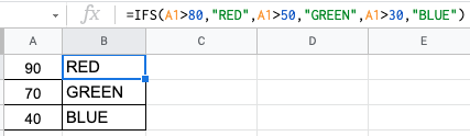
As you can see from the result, the function returns the value as RED when the score is 90, Green when the score is 70, and BLUE for 40.
Note:- You can use the IFS function for cells in range as well. Below is on example:
IFS({A1:A10}<80, “RED”, {A1:A10}<50, “GREEN”, {A1:A10}<30, “BLUE”)
Example-2:
Let’s see one more example of using the IFS function for nested if statements in google sheets.
Here we are trying to assign a project manager to our clients based on their billing hours.
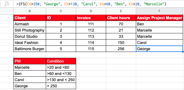
In the above example, we have 4 project managers. The second table tells us which PM to assign based on the number of hours.
So we have 4 conditions to check and we have used the IFS function to accommodate multiple IF statements.
You need to be careful when writing the conditions. Remember that the function checks them in a sequence from left to right.
Let’s say we check for the lowest hour first and assign a project manager. In this case, we may write the function like this,
IFS(E6 < 60, “Marcelle”, ………)
If we do that then all rows will have Marcelle’s name. You can try this yourself.
So we will start the function checking for the highest working hours.
=IFS(E1>250, "George", E1>130, "Carol", E1>60, "Ben", E>20, "Marcelle", true, "No PM needed")
The first test compares cell E1 to see if its greater than 250. If so, then it outputs “George”. If the first test fails, then the function checks the second condition. The second condition is to check if the cell value is greater than 130. If so, then it assigns Carol as the project manager. Next, it checks for greater than 60 and 20. It then outputs the result as “Ben” or “Marcelle”. If all the checks fail, then the IFS function will execute the default statement. For example, if the client hour is 10, then the default fallback condition is to output “No PM needed”.
If you change the order of the conditions inside the IFS function, then the output will be different. You have to be careful with the sequence of the conditions.
So the takeaway is that The IFS() function checks all conditions from left to right.
Notice one thing is that the Name of the PM is hardcoded in each of the conditions. This is generally not a good practice. Because it is hard to make a change in the future and also it is more error-prone.
A better solution to this problem is dynamic value picking. We can achieve this by modifying the formula like this
=IFS(E1>250, $B$12, E1>130, $B$11, E1>60, $B$10, E>20, $B$9, true, "No PM needed")
You can further enhance this formula by making the first condition values dynamic. Please try this yourself and see how you get there.
Here is the final solution sheet for your reference.
Let’s explore the IFs function in detail.
Return default when all IFS conditions fail
Let’s say I want a default value if all the condition checks fail in the IFS function. You can achieve this by adding the following condition,
= IFS(condition1, result1, condition2, result2, true, default)

Adding “true” and value at the end will show the default value if none of the IF conditions match.
IFS Formula Notes
- Like the IF function, the IFS function has 2 outcomes for a condition. It’s either TRUE or FALSE.
- In an IFS statement, there will always be one condition and its corresponding outcome. So IFS statements have an even number of arguments.
- The IFS function executes the logic from left to right. Meaning, if the first condition from left to right is true, then it will not execute further and stop there. So be sure when you write your conditions. Test them before finalizing the statement.
- Though technically there is no default value if all condition checks fail, you can create one. You can do so by adding a condition called “true” and defining its outcome as you wish to display.
IF Vs Nested IF Vs IFS
The IF function is one of the powerful logical functions in Google sheets. It checks the expression in a given cell and outputs true or false. When we want to check many conditions, we need a nested IF function.
We were using the nested IF function in google sheet for a long time for various manual calculations. Now we have switched to the IFS function in our daily work for all the logical calculations.
I am going to give you some real-life examples. I will explain how both options work. If you have been using nested IF formulas in a single cell, you will see how the IFS function is easy to write and use.
Below you have the syntax of IF formula, Nested IF formula and IFS formula listed.
=IF(logical_expression, value_if_true, value_if_false)

=IF(logical_expression, value_if_true, IF(logical_expression2, value_if_true2, IF(logical_expression3, value_if_true3, value_if_false)))

=IFS(condition1, value1, [condition2, value2, …])
Let us consider the same example of e-commerce website conversion data that we discussed at the start of this article.
We are trying to review the conversion rate of our web pages and identify which one to focus on.
We will use IF statement, Nested IF statement and IFS formula side by side.
Below are the 3 formulas we have used:
=IF(D2>5%,"Okay","Not Okay")

=IF(D2<1%,"Today",IF(D2<2%,"Tomorrow", IF(D2<4%,"Thursday",IF(D2<10%,"Friday","Error"))))

=IFS(D2<1%,"Today",D2<2%,"Tomorrow",D2<4%,"Thursday",D2<10%,"Friday")
Here is an example of all the 3 formulas in action.
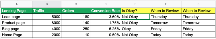
Column E outputs “Not Okay” if the conversion rate is less than 5% or it will out put “Okay”.
Columns F and G have the same purpose to tell us which web page to check on which day.
While Column F uses a Nested IF statement, column G uses the IFS function.
As you can see, the nested IF function has many parentheses compared to the IFS function. When you are trying to check a large number of conditions, the IFS function is easy to write, read and maintain.
FAQ
What are google sheets nested if statements?
Nested if statements in google sheets are used when you have multiple if statements to evaluate. You can nest all IF statements in one formula.
What is the google sheets nested if alternative?
IFS formula is the alternative to google sheets nested if.
How to avoid nested if statements in google sheets
To avoid nested if statements in google sheets, you can either simplify the IF statements or use the google sheets nested if alternative which is the IFS formula.
Final thoughts
The IFS statement is a powerful way to combine nested if statements in google sheets. While you can still use nested IF statements, the IFS function makes it more convenient.
Yet, when you start using both the IF and IFS functions, you will realize that these 2 functions alone can not solve complex problems. You need to combine the IF and IFS statement with functions like OR, ISBETWEEN, AND, SWITCH, etc.
Even more complex problems like working with ranges, columns, and other sheets need you to use a combination of other formulas. You need things like the ARRAY Formula, Vlookup, etc to solve them.
Appendix
[1] IFS formula in google sheets – Link
Further Reading
New to google sheets ? Start here
More related to Logical functions:
Logical functions in google sheets
Learn more about Google sheets Formulas.
Error handling in google sheets
